Command Line Interface Overview
The command line interface allows us to load and save States and run arbitrary functions on them.
Setup
To use the command line, we first define a package example containing the functions we want to run on the State:
example/lib.py
import numpy as np
import pandas as pd
from sklearn.linear_model import LinearRegression
from sklearn.model_selection import GridSearchCV
from sklearn.pipeline import make_pipeline
from sklearn.preprocessing import PolynomialFeatures

from autora.experimentalist.grid import grid_pool
from autora.state import StandardState, estimator_on_state, on_state
from autora.variable import Variable, VariableCollection

rng = np.random.default_rng()


def initial_state(_):
    state = StandardState(
        variables=VariableCollection(
            independent_variables=[
                Variable(name="x", allowed_values=np.linspace(-10, +10, 1001))
            ],
            dependent_variables=[Variable(name="y")],
            covariates=[],
        ),
        conditions=None,
        experiment_data=pd.DataFrame({"x": [], "y": []}),
        models=[],
    )
    return state


@on_state(output=["conditions"])
def experimentalist(variables):
    conditions: pd.DataFrame = grid_pool(variables)
    selected_conditions = conditions.sample(10, random_state=rng)
    return selected_conditions


coefs = [2.0, 3.0, 1.0]
noise_std = 10.0


def ground_truth(x, coefs_=coefs):
    return coefs_[0] * x**2.0 + coefs_[1] * x + coefs_[2]


@on_state(output=["experiment_data"])
def experiment_runner(conditions, coefs_=coefs, noise_std_=noise_std, rng=rng):
    experiment_data = conditions.assign(
        y=(
            ground_truth(conditions["x"], coefs_=coefs_)
            + rng.normal(0.0, noise_std_, size=conditions["x"].shape)
        )
    )
    return experiment_data


theorist = estimator_on_state(
    GridSearchCV(
        make_pipeline(PolynomialFeatures(), LinearRegression()),
        param_grid={"polynomialfeatures__degree": [0, 1, 2, 3, 4]},
        scoring="r2",
    )
)
example/__init__.py
# This __init__.py file is turns the `example` directory into a python package, allowing
# the other files plot.py and lib.py to import functions and variables from each other.
We can run the pipeline of initialization, condition generation, experiment and theory building as follows.
First we create an initial state file:
python -m autora.workflow example.lib.initial_state --out-path initial.pkl
Next we run the condition generation:
python -m autora.workflow example.lib.experimentalist --in-path initial.pkl --out-path conditions.pkl
We run the experiment:
python -m autora.workflow example.lib.experiment_runner --in-path conditions.pkl --out-path experiment_data.pkl
And then the theorist:
python -m autora.workflow example.lib.theorist --in-path experiment_data.pkl --out-path model.pkl
We can interrogate the results by loading them into the current session.
#!/usr/bin/env python
from autora.workflow.__main__ import load_state
state = load_state("model.pkl")
print(state)
# state =
# StandardState(
#     variables=VariableCollection(
#         independent_variables=[
#             Variable(name='x',
#                      value_range=None,
#                      allowed_values=array([-10.  ,  -9.98,  -9.96, ...,   9.96,   9.98,  10.  ]),
#                      units='',
#                      type=<ValueType.REAL: 'real'>,
#                      variable_label='',
#                      rescale=1,
#                      is_covariate=False)
#             ],
#         dependent_variables=[
#             Variable(name='y',
#                      value_range=None,
#                      allowed_values=None,
#                      units='',
#                      type=<ValueType.REAL: 'real'>,
#                      variable_label='',
#                      rescale=1,
#                      is_covariate=False)
#         ],
#         covariates=[]
#     ),
#     conditions=        x
#                342 -3.16
#                869  7.38
#                732  4.64
#                387 -2.26
#                919  8.38
#                949  8.98
#                539  0.78
#                563  1.26
#                855  7.10
#                772  5.44,
#     experiment_data=      x           y
#                     0 -3.16    1.257587
#                     1  7.38  153.259915
#                     2  4.64   54.291348
#                     3 -2.26   10.374509
#                     4  8.38  155.483778
#                     5  8.98  183.774472
#                     6  0.78    3.154024
#                     7  1.26   14.033608
#                     8  7.10  103.032008
#                     9  5.44   94.629911,
#     models=[
#         GridSearchCV(
#             estimator=Pipeline(steps=[
#                 ('polynomialfeatures', PolynomialFeatures()),
#                 ('linearregression', LinearRegression())]),
#             param_grid={'polynomialfeatures__degree': [0, 1, 2, 3, 4]},
#             scoring='r2'
#         )
#     ]
# )
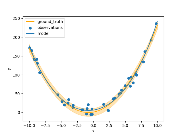
For instance, we can plot the results. We define another script in the example package:
example/plot.py
#!/usr/bin/env python
import pathlib

import numpy as np
import pandas as pd
import typer
from matplotlib import pyplot as plt
from sklearn.model_selection import GridSearchCV

from autora.state import StandardState
from autora.workflow.__main__ import load_state

from .lib import ground_truth, noise_std


def plot_results(state: StandardState):
    x = np.linspace(-10, 10, 100).reshape((-1, 1))
    plt.plot(x, ground_truth(x), label="ground_truth", c="orange")
    plt.fill_between(
        x.flatten(),
        ground_truth(x).flatten() + noise_std,
        ground_truth(x).flatten() - noise_std,
        alpha=0.3,
        color="orange",
    )

    assert isinstance(state.experiment_data, pd.DataFrame)
    xi, yi = state.experiment_data["x"], state.experiment_data["y"]
    plt.scatter(xi, yi, label="observations")

    assert isinstance(state.models[-1], GridSearchCV)
    plt.plot(x, state.models[-1].predict(x), label="model")

    plt.xlabel("x")
    plt.ylabel("y")

    plt.legend()
    plt.show()


def main(filename: pathlib.Path):
    state = load_state(filename)
    assert isinstance(state, StandardState)
    plot_results(state)


if __name__ == "__main__":
    typer.run(main)
... and invoke it on the command line:
python -m example.plot model.pkl
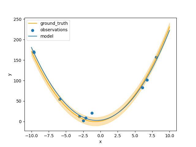
If we instead run the experiment for 4 cycles, we can get results closer to the ground truth.
set -x  # echo each command

python -m autora.workflow example.lib.initial_state --out-path "result.pkl"

for i in {1..4}
do
    python -m autora.workflow example.lib.experimentalist --in-path "result.pkl" --out-path "result.pkl"
    python -m autora.workflow example.lib.experiment_runner --in-path "result.pkl" --out-path "result.pkl"
    python -m autora.workflow example.lib.theorist --in-path "result.pkl" --out-path "result.pkl"
done

python example.plot result.pkl